|
Results

Box and whisker plot comparing the model's predictions with the observers' annotations, using Ground Truth Masks as a reference (click to enlarge).
Ground Truth Masks: From each test volume, 3 observers segmented the same 5 slices independently (capturing all 16 structures, n=59 total slices). From these annotations, a set of multi-rater consensus labels was constructed using STAPLE (12).
Statistical analysis: categorical linear regression with p<0.05.
Red asterisk: observer has higher Dice coefficients as compared to the model (p<0.05).
Green asterisk: observer has lower Dice coefficients as compared to the model (p<0.05).
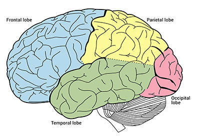
Blue asterisk: observer has higher Dice coefficients as compared to the model (p<0.05). However, the Ground Truth Masks contain a large number of slices that included the boundary between the temporal and parietal lobes, which is defined by an arbitrary straight line in the sagittal plane posteriorly. Overall Dice coefficients for the parietal and temporal lobes were higher when the model was evaluated on full volumes from the primary test dataset (see chart below).

Box and whisker plot comparing the model's performance between the primary and secondary test datasets (click to enlarge).
Red Boxes: Dice Coefficients of the model on the primary test dataset vs. Dice coefficients of the model on the iNPH dataset. Results from these datasets were analyzed together because both contained fully annotated volumes.
Blue Boxes: Dice Coefficients of the model on the Ground Truth Masks vs. Dice coefficients of the model on the RSNA dataset. Results from these datasets were analyzed together because both contained 5 annotated slices per volume representing all 16 structures.
Red asterisk: lower Dice coefficients as compared to the primary test dataset or Ground Truth Masks (p<0.05).
Green asterisk: higher Dice coefficients as compared to the primary test dataset or Ground Truth Masks (p<0.05).
Note: The model could not consistently identify the central sulcus in iNPH patients because ventricular enlargement severely distorted its appearance. Two volumes were excluded because the central sulcus could not be identified manually as well.
|
|
Citation
JC Cai, Z Akkus, KA Philbrick, A Boonrod, S Hoodeshenas, AD Weston, P Rouzrokh, GM Conte, A Zeinoddini, DC Vogelsang, Q Huang, BJ Erickson
“Fully Automated Segmentation of Neuroanatomy on Head CT Using Deep Learning”
Radiol Artif Intell. 2020 Sep; 2(5):e190183. https://doi.org/10.1148/ryai.2020190183
Click here to download citation data.
References
1. Frisoni GB, Geroldi C, Beltramello A, Bianchetti A, Binetti G, Bordiga G, et al. Radial Width of the Temporal Horn: A Sensitive Measure in Alzheimer Disease. Am J Neuroradiol [Internet]. 2002;23(1):35. Available from: http://www.ajnr.org/content/23/1/35.abstract
2. Diprose William K, Diprose James P, Wang Michael TM, Tarr Gregory P, McFetridge A, Barber PA. Automated Measurement of Cerebral Atrophy and Outcome in Endovascular Thrombectomy. Stroke [Internet]. 2019;50(12):3636–8. Available from: https://doi.org/10.1161/STROKEAHA.119.027120
3. Anderson RC, Grant Jj Fau - de la Paz R, de la Paz R Fau - Frucht S, Frucht S Fau - Goodman RR, Goodman RR, Neurosurg J. Volumetric measurements in the detection of reduced ventricular volume in patients with normal-pressure hydrocephalus whose clinical condition improved after ventriculoperitoneal shunt placement. (0022-3085 (Print)).
4. Toma AK, Holl E, Kitchen ND, Watkins LD. Evans’ Index Revisited: The Need for an Alternative in Normal Pressure Hydrocephalus. Neurosurgery [Internet]. 2011;68(4):939–44. Available from: https://doi.org/10.1227/NEU.0b013e318208f5e0
5. Relkin N, Marmarou A, Klinge P, Bergsneider M, Black PM. Diagnosing Idiopathic Normal- pressure Hydrocephalus. Neurosurgery [Internet]. 2005 Sep 1;57(suppl_3):S2-4-S2-16. Available from: https://doi.org/10.1227/01.NEU.0000168185.29659.C5
6. Kauw F, Bennink E, de Jong HWAM, Kappelle LJ, Horsch AD, Velthuis BK, et al. Intracranial Cerebrospinal Fluid Volume as a Predictor of Malignant Middle Cerebral Artery Infarction. Stroke [Internet]. 2019 Jun [cited 2020 Feb 19];50(6):1437–43. Available from: https://www.ahajournals.org/doi/10.1161/STROKEAHA.119.024882
7. Takahashi N, Shinohara Y, Kinoshita T, Ohmura T, Matsubara K, Lee Y, et al. Computerized identification of early ischemic changes in acute stroke in noncontrast CT using deep learning [Internet]. Vol. 10950, SPIE Medical Imaging. SPIE; 2019. Available from: https://doi.org/10.1117/12.2507351
8. Fritscher KD, Peroni M, Zaffino P, Spadea MF, Schubert R, Sharp G. Automatic segmentation of head and neck CT images for radiotherapy treatment planning using multiple atlases, statistical appearance models, and geodesic active contours. Med Phys [Internet]. 2014;41(5):51910. Available from: https://aapm.onlinelibrary.wiley.com/doi/abs/10.1118/1.4871623
9. Golby AJ. Image-Guided Neurosurgery [Internet]. Elsevier Science; 2015. 536 p. Available from: https://books.google.com/books?id=2v7IBAAAQBAJ
10. AI challenge [Internet]. [cited 2020 Apr 4]. Available from: https://www.rsna.org/en/education/ai-resources-and-training/ai-image-challenge
11. Warfield SK, Zou KH, Wells WM (2004). “Simultaneous truth and performance level estimation (STAPLE): an algorithm for the validation of image segmentation.” IEEE transactions on medical imaging, 23(7), 903–921.
12. Philbrick KA, Weston AD, Akkus Z, Kline TL, Korfiatis P, Sakinis T, et al. RIL-Contour: a Medical Imaging Dataset Annotation Tool for and with Deep Learning. J Digit Imaging. 2019/05/16. 2019;32(4):571–81.
13. Ronneberger O, Fischer P, Brox T. U-Net: Convolutional Networks for Biomedical Image Segmentation [Internet]. arXiv e-prints. 2015. Available from: https://ui.adsabs.harvard.edu/abs/2015arXiv150504597R
|


